The FIRE movement is built upon wrong assumptions

I am an optimist when it comes to my long term plans and a super pessimist when it comes to believing random success stories that I hear on the internet. The internet is a hotbed to amplify our survivorship bias. And knowing that there are probably billions of people on the internet, the single success stories have a chance of 1 in a billion to replicate for me. I am automatically very suspicious of any claim on the internet especially countless number of Canadians who arrived to wealth by moving down south to the US and investing their $75K tech incomes in VTSAX to retire in 5 years. I am not saying their story has not happened, but I strongly believe, considering that all of these success stories have interestingly happened during one of the longest bull markets in the US history, their story can be hardly replicated.

Additionally, just like any semi-successful trend, the FIRE movement has attracted a large number of opportunists who are coming to the movement to make a few bucks. There are a few examples of 25 year olds whose portfolio, if you calculate their true return, is returning way above 50% annual returns (remember Bernie Maddof? his guaranteed return was 20% and Benjamin Graham, the legendary investor whose book “The Intelligent Investor” has given rise to value investing, the legend who trained icons like Warren Buffet have had about 38% return in their best days). To these people add a few who have built an empire by walking dogs, sitting cats, and driving for Uber. God knows what brought wealth to the rest of these people, maybe hard work, maybe a trust fund, or cryptocurrency laced CBD

The compound interest formula:

Let’s for the sake of argument say we have $100, and would like to invest it in a high growth asset that grows 12% on average for 10 years. The formula to calculate the compound value is

If we plug in the numerical values after 10 years our 100 Dollar bill will grow into $310.58. A wonderful 310% growth. If you are lazy like I am, you can use one of the many compound interest calculators online to arrive at this exact number

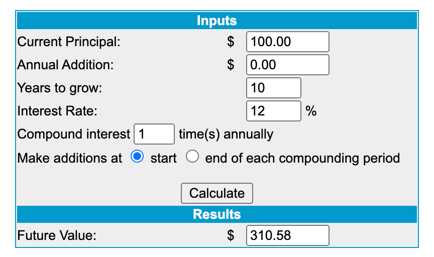
This means that if I have $1M, I can probably safely Fat FIRE in 10 years even if I work as a barista for the next 10 years to pay the bills while the army of my little Dollar bills is growing to $3.1M to earn me retirement for the rest of my life.

But average growth is the most optimistic scenario

What people don’t tell you is that this number is pretty much the best case scenario. It is essentially the optimal performance of your portfolio that completely ignores market volatility. Let me show you why. Let’s for the sake of argument imagine we are looking at an average of 12 percent growth over a short 2 year horizon. Also consider the following four scenarios which all have the average 12% growth but you will end up with different amount of assets at the end:

Scenario one:

• Year 1: 12%
• Year 2: 12%
• Future Value: $125.44

Scenario two:

• Year 1: 0%
• Year 2: +24%
• Future Value: $124

Scenario three:

• Year 1: -12%
• Year 2: +36%
• Future Value: $119.68

Scenario four:

• Year 1: +36%
• Year 2: -12%
• Future Value: $119.68

See, all of these scenarios have the same average growth over the 2 year horizon but the market volatility goes up significantly in the scenarios 2,3, and 4. In fact as the market volatility goes up your portfolio starts to perform worse.

As volatility goes up your FIRE dreams fall apart

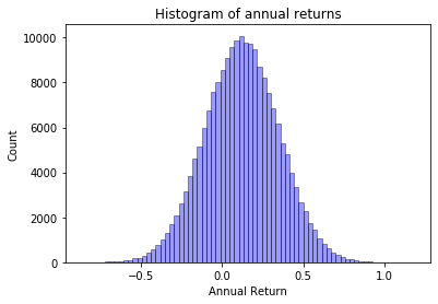
Let’s build a small simulator to estimate our portfolio’s return in various regimes of volatility. I assume that my portfolio can produce a return between -100% to 300% every year and this return is normally distributed around the mean of 12%. This way I can vary the standard deviation of the samples as estimate my portfolio returns more realistically.

The following little Python script generates random returns that are between -100% and 300% whose mean is exactly 12%

import numpy as np 

# Generates t returns with average of mu
def generate_seq(min_val, max_val, mu, t, sigma):
    s = np.random.normal(mu, sigma, t)
    s = [min(max(x, min_val), max_val) for x in s]
    mean_val = np.mean(s)
    diff = mean_val-mu
    s = [x-diff for x in s ]
    return s
   
# Convenient wrapper for generate_seq
def generate_my_seq():
    return generate_seq(-1.00, 3.00, .12, 10, .24)
d = generate_my_seq()
print(d)
print(np.mean(d))

As sample sequence of returns produced by this code will be

[0.4636707418453361, -0.015194351776261508, 0.12141853784353404, 0.19838200461651365, 0.20743710814249752, 0.4447197851379031, 0.24032558821925656, -0.22403723286831953, 0.03366595856070387, -0.2703881397211638]

That results in the exactly 12% average return

I can visualize the distribution of these returns using a simple code like this

vals = []
for j in range(0, 20000):
    for i in generate_my_seq():
        vals.append(i)

# Import the libraries
import matplotlib.pyplot as plt
import seaborn as sns

# seaborn histogram
sns.distplot(vals, hist=True,kde=False,
             bins=int(360/5), color = 'blue',
             hist_kws={'edgecolor':'black'})
# Add labels
plt.title('Histogram of annual returns')
plt.xlabel('Annual Return')
plt.ylabel('Count')
print(np.mean(vals))
print(np.std(vals))

I can now run my simulator for various values for volatility and calculate my final portfolio value

sims = 200000
init = 100 


for sigma in [x*a for x in [0, .25, .5, .75, 1,2,3,4,5,6]]:
    vals = []
    for i in range(0, sims):
        d = generate_seq(-1.00, 3.00, a, t, sigma)
        y = init 
        for j in d:
            y+= y*j
            if y<0:
                y=0
        vals.append(y)


    # seaborn histogram
    plt.figure()
    sns.distplot(vals, hist=True,kde=False,
                 bins=int(360/5), color = 'blue',
                 hist_kws={'edgecolor':'black'})
    # Add labels
    plt.title('Histogram of final values')
    plt.xlabel('Compound Value')
    plt.ylabel('Count')
    print("-----")
    print("sigma:", sigma)
    print("mean:", np.mean(vals))
    # print(np.std(vals))
    print("min:", min(vals))
    print("max:", max(vals))
    #sorted(vals[-10:])
    #sorted(vals[:10])
    print("\n\n\n")

For zero volatility I arrive at my rosy FAT FIRE picture that the compound interest calculator gives me, I can fat fire in 10 years without any worries. All of those FIRE conferences were right, retiring on a $75K salary is so easy.

sigma: 0.0
mean: $310.58

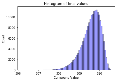
However as I increase the standard deviation (volatility) of the returns my retirement slips away from my hands. Below is the results for the 3% volatility

sigma: 0.03
mean: $309.58
min: $306.22
max: $310.52

Still not bad, in the worst case scenario if the volatility is only 3% I will be able to retire with $306 dollars ($3.06M for my $1M portfolio), and the distribution of final values looks something like this (less variety on the upside and more chance of longer tail on the downside)

For an slightly more realistic case of having 12% standard deviation, I get the following. On average I will still have about $2.9M but I might end up with $2.4M and my best case scenario will never reach the FIRE calculator’s $3.1058M

sigma: 0.12
mean: $294.814
min: $242.329
max: $310.234

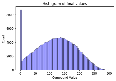
And if we have a 48% sigma I will have a large chance of going broke at the end of 10 years (look at the large bar on 0$ in the following graph)

sigma: 0.48
mean: 120.86
min: 0.0
max: 301.50

So what does it mean?

This doesn’t mean you shouldn’t invest. It doesn’t even mean you cannot Fat FIRE in 10 years. But what it tells you is that your friendly compound interest calculator is giving you the most optimistic scenario and you should not rely on it. For my retirement calculation I will probably use a more realistic 7 to 8% return with a volatility of 12%. Sure it means that I probably have to work for 3 more years.

Another thing that you need to know is that here we have used a long time horizon of 10 years and as time goes by you can recalculate your portfolio return to arrive at a tighter estimate for your retirement. Your estimate at year 9 is going to be more accurate than your estimate at year 0.